It’s been a while since I wrote about my Model Justice project, which is an attempt to build a software model of certain aspects of the criminal justice system. In my last post on the subject, I explained why I was abandoning the Insight Maker systems modeling environment in favor of the Python general-purpose programming language. Since then, I’ve been slowly climbing the learning curve, and even though I haven’t quite caught up to the Insight Maker based implementation, I think I’m at a point where I can begin talking about it.
My goal with this Python rewrite is not to build a single monolithic criminal justice simulation program. As I’ve emphasized from the start, this project is about learning and exploration, and I haven’t yet learned enough to build an all-in-one solution like that. Rather, I’m writing a collection of Python components — classes in software terminology — that I can assemble and configure in various ways to build a variety of models.
For my purposes, the basic unit of simulation is the Case class, which represents a single criminal case, consisting of a single criminal charge against a single defendant, making its way through the criminal justice system. Each Case entering the system has two basic parameters which describe it:
prob_convict: A number between 0 and 1 inclusive, representing the probability of a conviction if the case goes to trial.sentence_if_convicted: A number indicating the length of the sentence the judge will impose if the defendant is convicted by the trial. This is a unitless value, but I tend to think of it as months.
Cases are grouped together by the Docket class. Each Docket represents a group of cases that are being considered at the same time. The simulation creates one Docket for each iteration of the simulation by calling a DocketFactory class, which itself uses a CaseFactory class to create each of the Cases it puts in the Docket. The CaseFactory class, in turn, uses a random number generation class to generate the prob_convict value for each case. (The sentence_if_convicted value is currently hardcoded at 60 until I implement a better way to generate it.) The DocketFactory class itself uses a random number generator to decide how many Cases to put in each Docket it creates.
(I’ve included three random number generator classes, each providing a different distribution, any of which can be used by a factory class.)
Currently, the simulation is so simple that this grouping of Cases into Dockets has no effect on the outcome, but in the future I hope to use the Docket class to implement the court system’s resource limits and decision making horizon. For example, if there are only enough courtrooms to hold 20 trials per simulation cycle, but 30 cases are on the docket, then the simulated decision makers will have to resolve the remaining 10 cases by some other means, such as plea bargaining or dismissal.
It would have been simpler to have the main simulation code create a Case or a Docket whenever it needed one, but then I’d have to change the main code each time I wanted to run a different simulation with different parameters. Since I’d rather keep the core simulation code stable, I put the code for Case and Docket creation in corresponding CaseFactory and DocketFactory classes that the simulation can invoke when it needs a Case or a Factory. This allows me to change the parameters of the simulation by changing the factory classes without having to change any of the other code in the simulation. This is called a factory pattern, and it’s a good way to write flexible software.
At the top level of the simulation is the Experiment class, which actually runs the simulation engine. Constructing a new Experiment takes three parameters:
- A DocketFactory object which it uses to create dockets and cases,
- a PleaBargainingStrategy object which specifies how plea bargaining decisions are made, and
- a Trial object which simulates the trial outcome.
I’ve already discussed the DocketFactory, but the other two classes are new.
The PleaBargainingStrategy object processes each Docket of cases and figures out which cases will settle with plea bargains and which ones will go on to trial. In the future, I hope to have subclasses that implement a reasonably plausible model of the plea bargain process, but for now all I have is PleaBargainingAtRandom, which implements a dumb algorithm that chooses what to do with each case entirely at random. E.g. if you set its prob_plea parameter to 0.9, the strategy will randomly generate a plea deal 90% of the time. The deal will always be for a sentence that is the mathematically expected length: If prob_convict on a case specifies a 30% chance of conviction, and the sentence if convicted is 60 months (which it always is right now), then the plea deal will be for a sentence of 0.3 * 60 = 18 months.
The Trial class is even simpler: It generates a uniform random number between 0 and 1, and if it’s less than prob_convict the defendant is found guilty and serves the full sentence. Otherwise the defendant is acquitted and does no time.
Those are the pieces that make up a simulation of how cases work through the criminal court system. To show how the pieces come together, let’s walk through a script that runs an experiment.
(If you’re a Python user, you can follow along by installing the crimjustsimpy package in your Python environment. If you are reading this some time after I published it, I may have released newer versions which work differently, so to get the package this post is talking about, make sure to specify version 1.0.5. If you’re interested, the source code for this project is also available on GitHub, and you can specifically view release 1.0.5.)
The sample script starts by defining some parameters at the top:
AVG_CASES_PER_INTERVAL = 100
MAX_CASES_PER_INTERVAL = 300
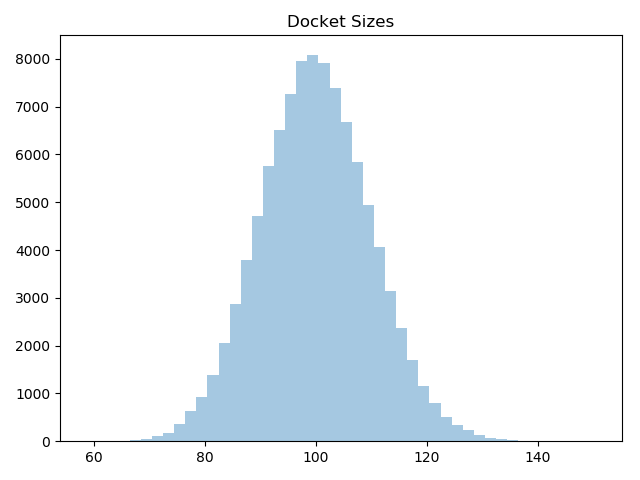
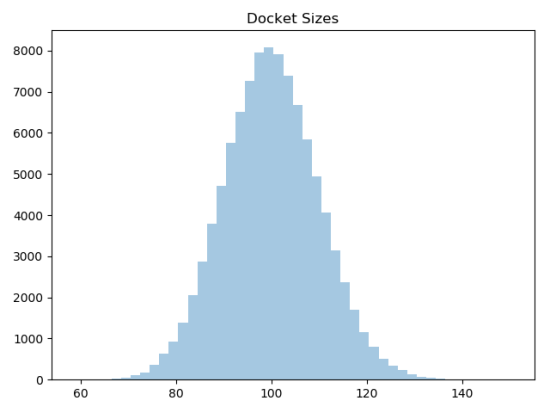
The number of cases to be generated for each docket is specified by a Poisson distribution, which is a common distribution used to estimate the arrival rate for random independent events, where each one has the same probability of occurring over a given time period. It’s commonly used to simulate things like orders arriving at a warehouse or cars arriving at a gas station. In this case, we’re assuming an average arrival rate of 100 cases per simulation interval.
Although large numbers (relative to the average) would be very rare, the Poisson distribution places no upper limit on the number of cases that can arrive during the interval. To avoid insane outliers, we’re limiting arrivals to a maximum of 300. That’s probably not necessary, because you can see in this histogram of a sample of 100,000 dockets shows, it never gets close to 300:
The next three lines describe the probability distribution from which probabilities of conviction will be drawn.
MIN_PROB_CONVICT = 0.05
MEAN_PROB_CONVICT = 0.4
MAX_PROB_CONVICT = 0.95
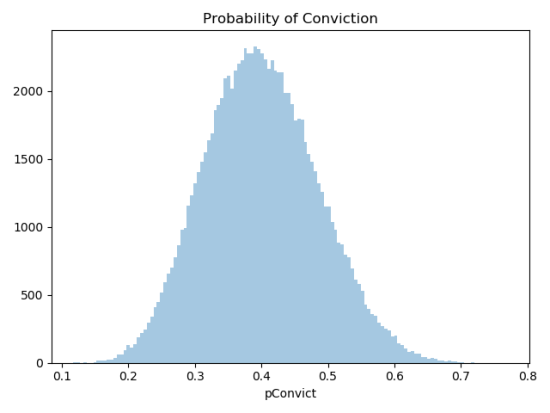
In my first attempt, I used a normal distribution with upper and lower limits. This time around, I’m using a beta distribution. I chose it because it has a nice shape, similar to the normal curve, but it also generates values in a strict range of 0 to 1 without the need to impose external cutoffs. As you can see, the configured range only runs from 0.05 to 0.95, so neither a conviction nor an acquittal is ever a certainty. The beta variate is internally scaled to fit withing these limits. Moreover, the beta distribution appears to be a good choice for representing a probability distribution from which to draw probabilities, which is exactly what I’m using it for.
The resulting histogram of conviction probabilities looks like this:
 The next parameter just tells the simulation what probability to use when deciding whether a case will end in a plea deal. This example uses 80%:
PROB_PLEA=0.8
Finally, we specify the number of iterations over which the model will cycle.
ITERATIONS = 240
After that, the script begins constructing and assembling the parts of the experiment. First, it creates a random number generator object that uses the Beta distribution to generate the conviction probabilities for the cases:
convict_gen = cj.RandomScaledBetaProb(
    shape=10.0,
    lower=MIN_PROB_CONVICT,
    middle=MEAN_PROB_CONVICT,
    upper=MAX_PROB_CONVICT)
RandomScaledBetaProb is a wrapper around the Python library function that generates the Beta distribution, specifying the bounds and the mean of the generated values. The shape parameter controls how tightly the numbers cluster around the mean or stretch out to the edges. I just picked 10 because it gives a nice looking curve. It should probably be a parameter in the future.
The next line of the script creates a CaseFactory from the conviction probability generator:
case_factory = cj.CaseFactory(convict_gen=convict_gen)
(If you’re unfamiliar with Python named parameters, that probably looks a little confusing. In “convict_gen=convict_gen“, the first “convict_gen” is the name of the CaseFactory parameter that receives the conviction probability generator, and the second “convict_gen” is a reference to the variable that received the conviction probability generator created in the previous code snippet. This is a common coding convention.)
The next two lines do the same thing for the DocketFactory class. First create the object that generates the arrival rates for the dockets over the Poisson distribution, then create the DocketFactory itself, passing it the CaseFactory we created above and the arrival rate generator created here.
arrival_gen = cj.RandomPoissonBounded(
    mean=AVG_CASES_PER_INTERVAL,
    upper=MAX_CASES_PER_INTERVAL)
docket_factory = cj.DocketFactory(
    case_factory=case_factory,
    arrival_gen=arrival_gen)
The plea bargaining strategy is pretty simple, because it only takes the single value representing the probability of handling the case with a plea deal.
plea_bargaining = cj.PleaBargainingAtRandom(prob_plea=PROB_PLEA)
The trial is even simpler:
trial = cj.Trial()
Now we can assemble all these pieces to build an Experiment object:
experiment = cj.Experiment(
    docket_factory=docket_factory,
    trial=trial,
    plea_bargaining=plea_bargaining)
That brings us to the meat of the simulation: Running the experiment.
data = experiment.run(ITERATIONS)
It’s just one line, but it does all the work of creating the dockets filled with cases, resolving some of them with plea deals, resolving the rest with trial, and gathering up the results. With only 240 dockets and and 100 cases per docket, this runs in less than a second on my computer. In the future, with more cases and more complicated resolution logic, it will probably run a lot longer.
The results of the simulation run are returned in an ExperimentData object that contains all the Docket and Case objects with the results of all the cases. There’s nothing to stop us from traversing the Case objects directly, but there’s a better way:
df = data.casesToDataFrame()
This converts the Case data to a DataFrame, which is a highly-optimized standard Python data structure for handling tabular data. This will make it easier to process the data in the future, because lots of Python code packages understand how to work with DataFrames. For example, the PyCharm development environment I use can render DataFrames as tables:
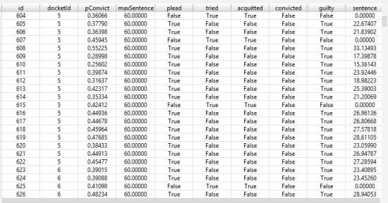 This shows the output from a simulation run for each case. The fields are defined as follows:
id: A unique integer ID assigned to each case.docketId: A unique integer ID indicating the docket the case belonged to.pConvict: The probability of conviction of the case when created.maxSentence: The maximum possible sentence if convicted.plead: True if the case was handled with a plea deal.tried: True if the case was decided with a trial.acquitted: True if the defendant was acquitted at trial. Always False if the case didn’t go to trial.convicted: True if the defendant was convicted at trial. Always False if the case didn’t go to trial.guilty: True if the defendant was convicted at trial or if the defendant took a plea deal.sentence: Actual resulting sentence. Always 0 if the defendant was acquitted.
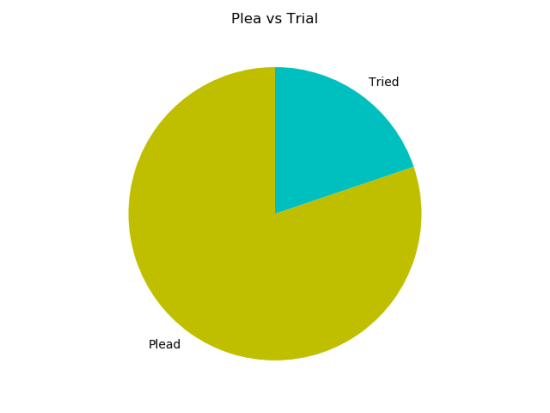
We could plot this data using standard Python graphics packages such as matplotlib and seaborn, but the crimjustsimpy package also includes a Visualization class that collects a handful of convenience methods for creating plots from the DataFrame. For example, this pie chart showing the ratio of cases that plead out vs. going to trial:
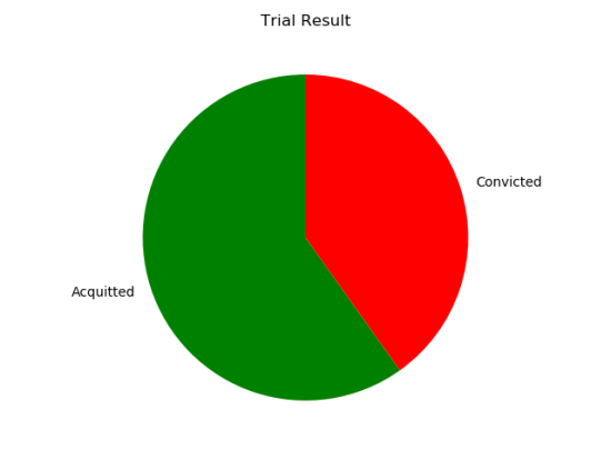
This is how the trials turned out:
And this is a breakdown showing all three possible case results: Acquitted at trial, convicted at trial, and plead out: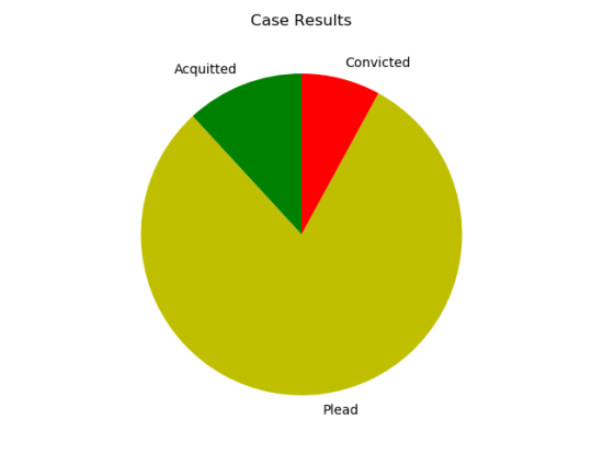
None of that is particularly surprising. We set up the simulation to take a plea deal 80% of the time, and it did. We set it up for 40% of trials to result in convictions, and they did. We’re just confirming that the simulation ran the way we wanted it to.
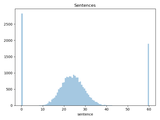
It’s slightly more interesting to plot a histogram of the lengths of the resulting sentences for all the cases:
That looks a little weird, but it makes sense. The hump in the middle is showing the sentences from the plea deals, all of which are for the maximum sentence weighted by the probability of conviction, so they follow the same beta distribution hump as the probability of conviction. The bars at the ends are all the cases that went to trial, because they ended with either no sentence or the maximum sentence. The difference between the plea hump and the conviction bar on the right is what defense lawyers call the “trial tax.” It’s the difference between what happens when a defendant admits guilt, and what happens when he makes the government prove it.
That’s about all I’ve got done so far, other than some unit tests and a few sample scripts, which leaves me a lot more to do.
The previous version of this model used an agent-based systems model that tracked the changing state of the cases over time as they worked their way through the system. That was interesting to see, and it gave me the simulated steady-state size of the prison population, which seems like an important metric for studying criminal justice.
I’d like to put that output capability back into the model, but I’m not sure if I should keep a running track of the state of each case like last time, or if I should just run a post-pass to compute time series data for the prison population from the case results.
I’d also like to be able to see intermediate results from the simulation, either by having it generate usable output as it runs, or by being able to run it for a few iterations and then stop to examine what it’s doing. This suggests that keeping a running state will work better than a post-pass analysis.
In addition, if I can stop and start the simulation, I’d also like to be able to change the parameters while it’s stopped, so I can model changes to the system. This suggests I need to break down the Experiment class into at least two parts: The simulation engine, which can be modified along the way, and the simulation data, which persists throughout the simulation run.
Of course, none of that helps me with what I really want to look at, which is the plea bargaining decision. I have some ideas about that, but this post is long enough.
As always, any suggestions would be appreciated.

One factor that may influence whether a defendant will accept a plea deal is whether they have been in jail before and whether they are prepared to do time again. Most everyone abhors going to jail, but if you have been there before and there is nothing special for you on the outside, doing the time might be an acceptable result. I have no idea how you might model this, but I am confident you will think of something. (I think that’s a line from a movie somewhere.)
Interesting thought. I wasn’t planning to model things like that beyond maybe a parameter that quantifies a defendant’s willingness to risk jail. I think what you’re talking about would just fold into that parameter. However, if I modeled defendants individually and accounted for those who made multiple trips through the system, there might be a feedback effect, where imprisoning lots of people creates a population that is tolerant to being imprisoned… That might be interesting.
Nice project, I got a huge database of criminals, I am planning to implement a similar model, to judge actual crime probability.